Physical Intelligence is bringing general-purpose AI into the physical world.
π 系列堪称经典。前段时间实践了 π0 的真机部署与加速,最近又做了 π0.5 的仿真,感觉是时候系统整理一波了。
π 相关背景
2025-02-04 — π0:Physical Intelligence 的首个 First Generalist Policy,面向通用操控的机器人基础模型,常被视作该系列的奠基之作。
- 从预训练的视觉-语言模型(VLM)出发,继承互联网规模预训练带来的语义与视觉表征;借助流匹配(flow matching,可视为扩散的一类变体)输出连续动作。
- 典型结构
- 双专家:VLM 专家 + 动作专家(action expert)分工协作;
- 流匹配:用向量场 / 去噪视角建模动作分布,与 VLM 侧表征对齐。
2025-04-22 — π0.5:泛化与任务分解能力更强;官方表述为迈向更普及具身智能(embodied intelligence)的重要一步。
- 双专家交互重构
- 动作专家去掉本体感知状态作为独立输入,专注于动作序列建模;
- 引入高层语义推理模块,可把抽象指令(例如「整理厨房」)拆解为子任务链(例如「拾取餐盘 → 丢弃垃圾」)。
- 数据:在异构数据上做共训练(co-training on heterogeneous data)。
- 双专家交互重构
2025-11-17 — \(\pi^{*}_{0.6}\)(Learns from Experience):强调从经验中学习的 VLA。
- 规模:VLM 主干约 2.6B → 4B,动作专家约 300M → 860M,以容纳更丰富的异构 prompt / 条件信息。
- RECAP:基于优势条件策略的离线 RL 框架;官方叙事里将其与机器人的自我纠错、以及在部分任务设定上相对人类演示的策略超越一并强调。
- 注:\(\pi^{*}_{0.6}\) 比较特殊的是还带了 star,意思是用了强化学习,类似 \(Q^{*}\)。
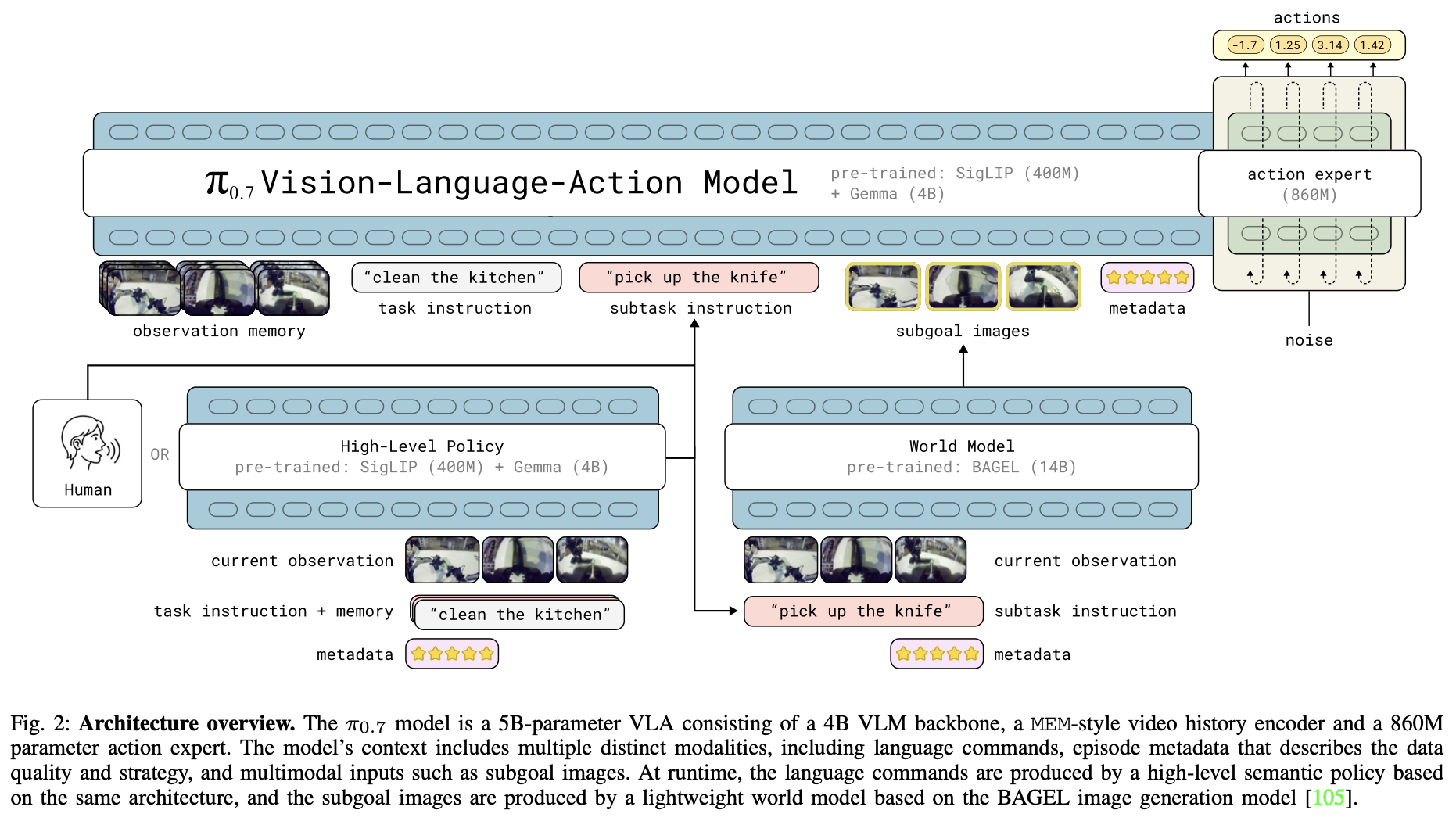
2026-04-16 — π0.7:官方称为具有涌现能力的可引导模型(A Steerable Model with Emergent Capabilities)。
- 多路输入(相较前代更细):
observation memory、task instruction、subtask instruction、subgoal images。observation memory(图像 448×448)- 最多 4 路图像;每路最多 6 帧历史(经视觉编码后参与注意力)。
- 历史帧经 vision encoder 处理,在 token 数量上压缩到与单帧相当,再送入主干。
subtask instruction- 先由 VLM 做一轮推理,得到子任务级文本指令。
subgoal images(448×448)- 由约 14B 的 BAGEL world model 生成中间「子目标」画面;
- 最多 3 张,与观测图像共用同一套图像编码器。
- 多路输入(相较前代更细):
模型结构
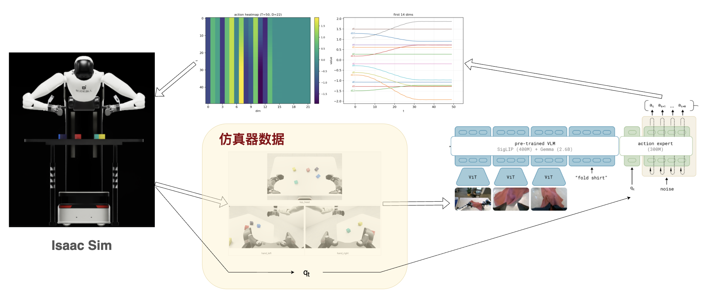
以经典的 π0 framewaork 为例:
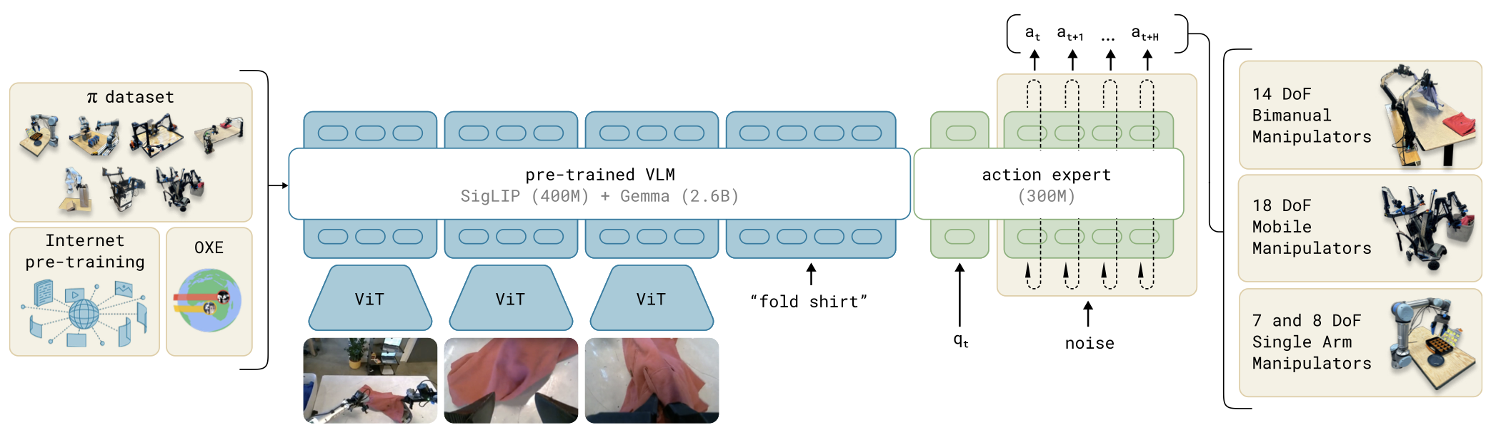
该模型由一个较大的视觉-语言模型(VLM)骨干网络,以及一个较小的、用于处理机器人状态和动作的动作专家(action expert)模块组成。 VLM 骨干网络的权重初始化自 PaliGemma,从而继承了大规模互联网预训练所学习到的表示能力。
┌──────────────────────────────┐
│               actions        │
│               ▲              │
│              ┌┴─────┐        │
│  kv cache    │Gemma │        │
│  ┌──────────►│Expert│        │
│  │           │      │        │
│ ┌┴────────┐  │x 10  │        │
│ │         │  └▲──▲──┘        │
│ │PaliGemma│   │  │           │
│ │         │   │  robot state │
│ │         │   noise          │
│ └▲──▲─────┘                  │
│  │  │                        │
│  │  image(s)                 │
│  language tokens             │
└──────────────────────────────┘整体是「视觉 + 语言 +
动作」三路:V 为 SigLIP 图像编码;L 为
Gemma 系语言 backbone;A 为
flow matching 的 action expert(与 VLM 通过 kv
kache 交互,即 Cross-Attention)。
| 模型 | V(SigLIP) | L(Gemma) | A(action expert) | 合计(约) |
|---|---|---|---|---|
| π0 | 400M | 2.6B | 300M | ~3.3B |
| π0.5 | 400M | 2.6B | 300M | ~3.3B |
| \(\pi^{*}_{0.6}\) | 400M | 4B | 860M | ~5.3B |
| \(\pi_{0.7}\) | 400M | 4B | 860M | ~5.3B |
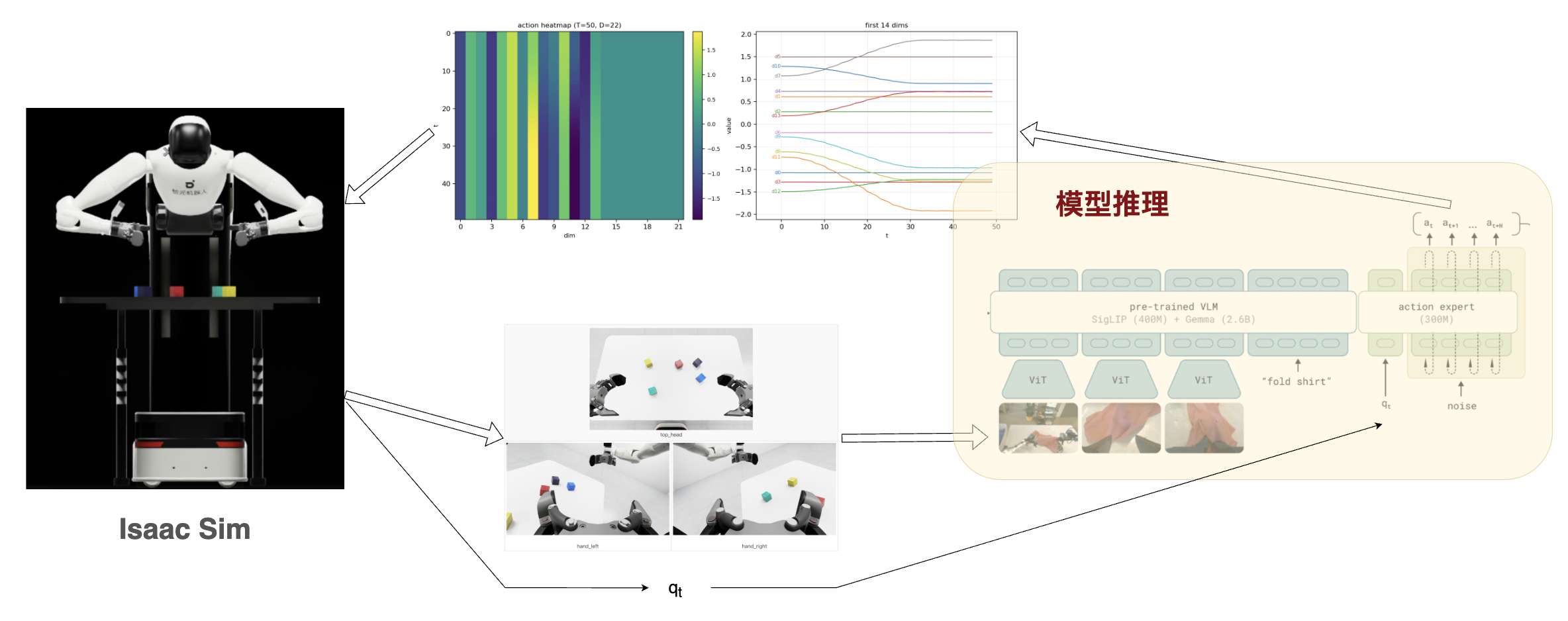
实践
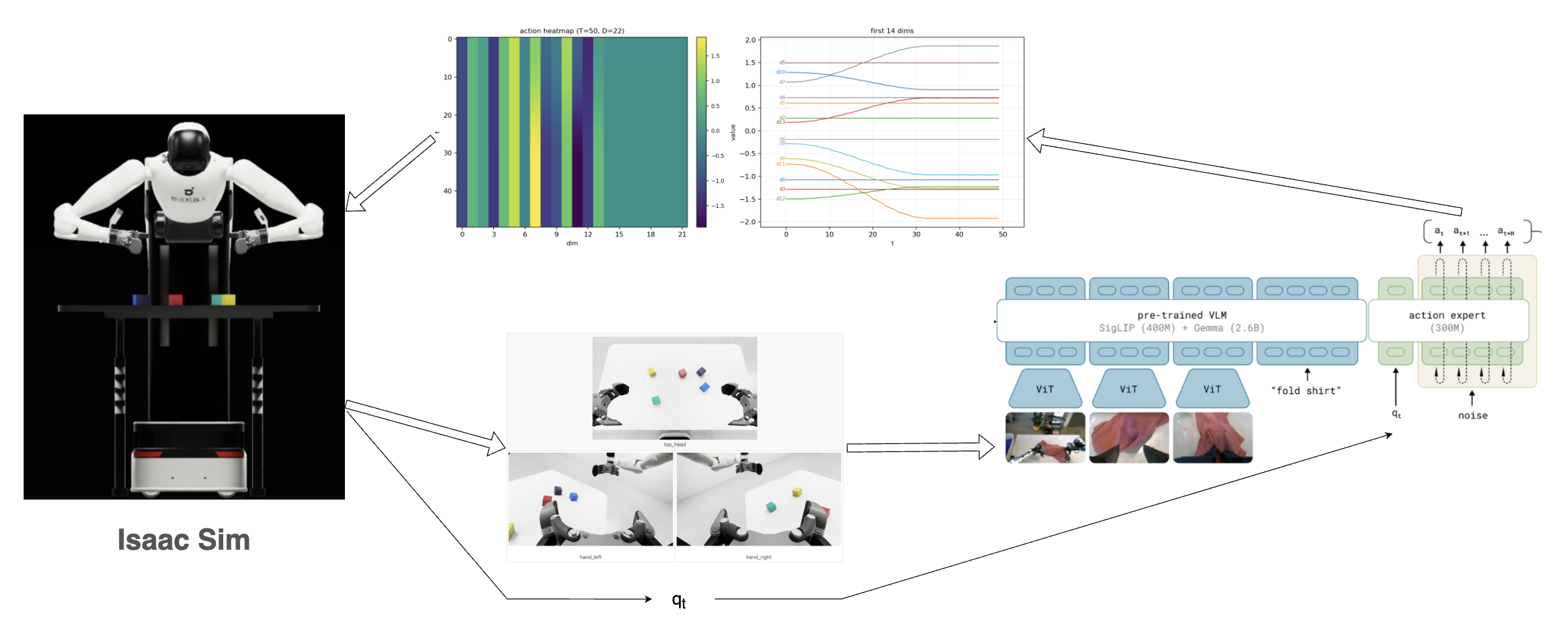
整体是使用了 NVIDIA Isaac Sim 进行仿真,使用 LeRobot 进行 π0.5 模型的推理,实现了捡桌子上某个颜色方块的任务。
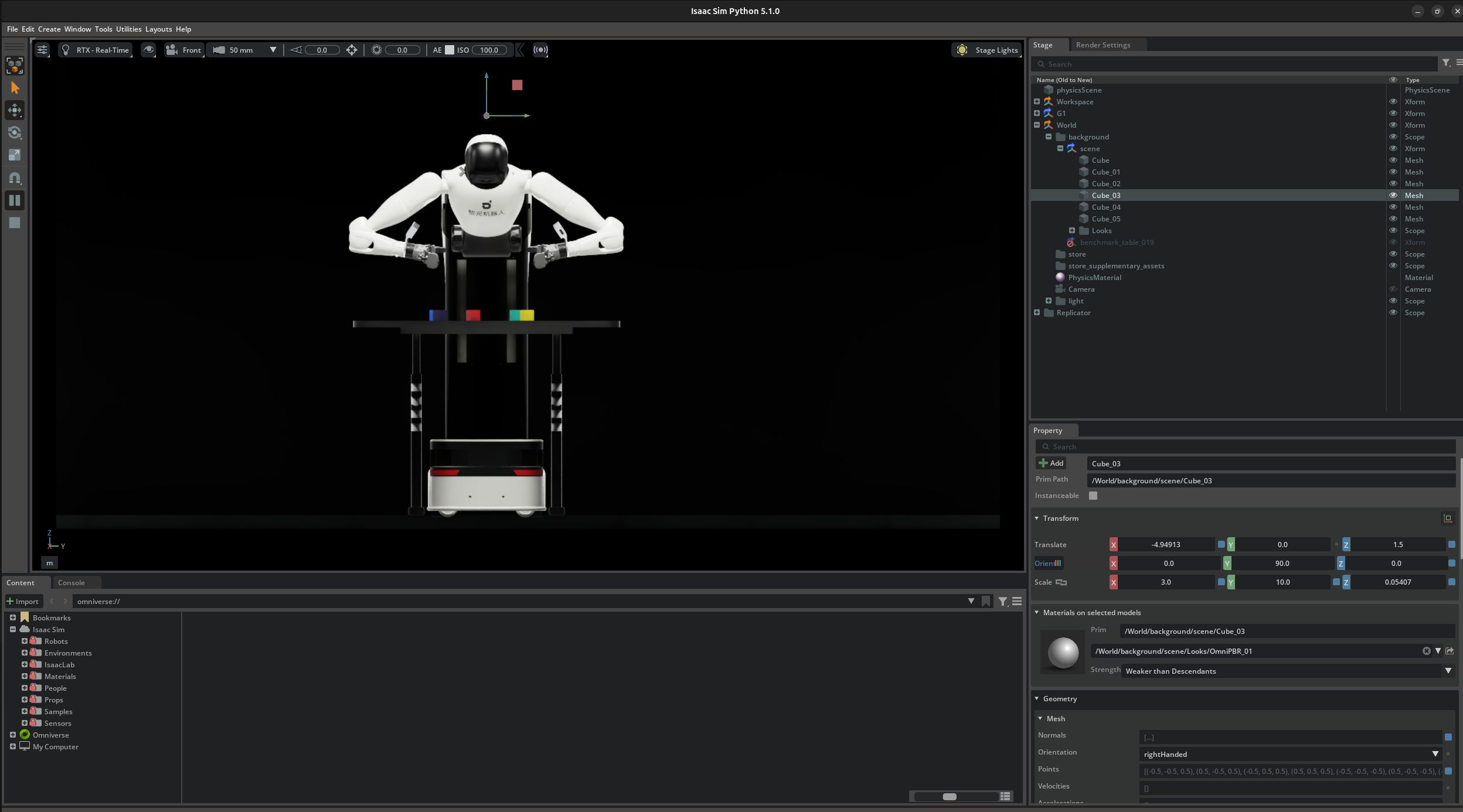
仿真器
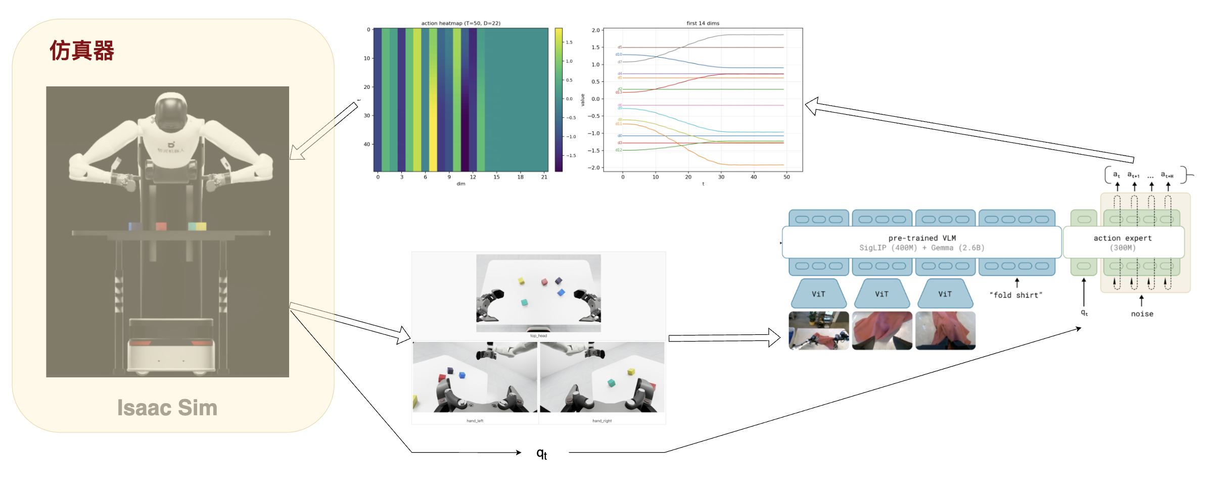
仿真器使用了 NVIDIA Isaac Sim,按照Genie Sim 3.0 进行了搭建。
Launch docker container and run the demo
1 | omni_python source/geniesim/app/app.py --config ./source/geniesim/config/select_color.yml |
初始化log
展开查看完整初始化日志(左臂 + 右臂 Solver)
1 | ========== 初始化 Solver ========== |
G1 机器人逆解(IK)求解器 的配置位于
source/geniesim/utils/IK-SDK/g1_solver.yaml
从 joint_space 里面可以看出, 关节顺序是
肩 3 + 肘 1 + 腕 3 1
2
3
4
5
6
7
8
9
10joint_space:
Weight coefficients for each joint; larger weights indicate less preference to move these joints
weights:
joint_1: 1.2 # Shoulder joint
joint_2: 1.2 # Shoulder joint
joint_3: 1.2 # Shoulder joint
joint_4: 1.0 # Elbow joint
joint_5: 1.0 # Wrist joint
joint_6: 1.0 # Wrist joint
joint_7: 1.0 # Wrist joint
完成仿真器启动
这个仿真器在
source/geniesim/utils/comm/websocket_client.py
中实现了一个通过 WebSocket
调用远端策略(policy)的客户端,让本地仿真/控制端像调用本地模型一样发观测、收动作。
1 | def infer(self, obs: Dict) -> Dict: # noqa: UP006 |
解析:若尚未连接则先连上远端 WebSocket,把 obs 用 msgpack 打包发过去,再把收到的字节 unpackb 返回。
推理服务端
推理端接收到仿真器数据(obs),进行图像预处理后进行模型的推理,生成对应的action。
接收仿真器数据
1 | obs (dict, len=5) |
state是一个 shape 为(32,)的状态向量- 主要用于编码机器人当前的 joint 状态;
- 在本次实践中,该向量存在一定冗余,主要有效信息集中在前 16 维(左臂 7 维 + 右臂 7 维 + 2 个夹爪维度)。
- 如果机器人存在更多的关节或者机械臂,会使用更多的维度。
- 需要注意的是,上图中引用的 \(\pi_{0}\) 的图,state 是送到了 action 模块,输出绝对动作
eef是 End-Effector 的缩写,也就是“机械臂末端执行器”状态eef 存的是左右手(夹爪/末端工具)的实时空间位姿。
Joint 是关节怎么动,EEF 是末端在哪、朝哪。
Joint EEF 变量 各关节角 (q) 末端位姿(位置、姿态) 空间 关节空间 笛卡尔 / 任务空间 二者关系: 通过 正运动学,由 (q) 得到末端位姿;逆运动学是由期望末端位姿反求 (q)(本 YAML 即在配置该 IK 优化问题)
在本次实践中,没有用到该数据(个人感觉其实用这个数据应该更合理一些?)
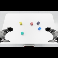
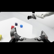
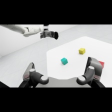
images表示机器人当前观测到的多视角图像信息- 包含头部相机、左腕相机和右腕相机三个视角。
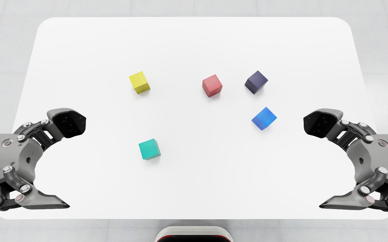 top_head top_head
|
|
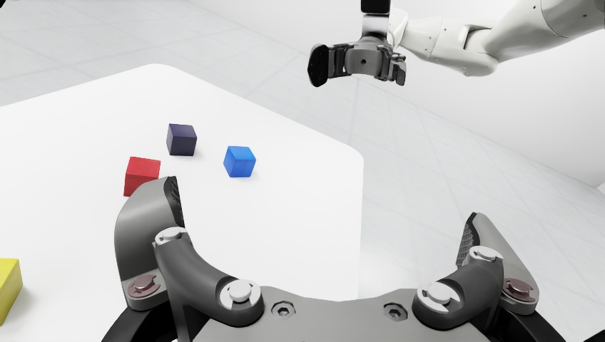 hand_left hand_left
|
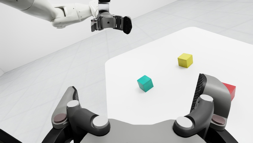 hand_right hand_right
|
prompt:任务提示词(例如"right arm picks up the red block on the table");- 在仿真 benchmark 中,该字段用于定义当前回合的目标任务(如 red/blue/yellow block 等不同目标);
- 在实际推理阶段,也可以替换为自定义指令,用于测试模型在不同语言目标下的泛化能力。
服务端预处理
服务端将图像转换为 float 类型,将 prompt
转换为 token,于是从仿真器接收的数据 obs
转换为以下格式的 batch:
infer batch:
1 | action: None |
将以上数据 batch: dict[str, Tensor] 发送至 LeRobot
进行infer
模型推理接口:select_action
vs predict_action_chunk
推理阶段主要有两个接口,语义分别是“拿一步动作”和“拿一段动作”:
1 | def select_action(self, batch: dict[str, Tensor]) -> Tensor: |
select_action:返回当前时刻的一步动作;predict_action_chunk:一次返回一个 action chunk(多步动作序列),适合加入 RTC 逻辑。
在本文实验中,调用 predict_action_chunk 获取一个 chunk
的 actions,返回给仿真器。
1 | def predict_action_chunk(self, batch: dict[str, Tensor], **kwargs: Unpack[ActionSelectKwargs]) -> Tensor: |
预处理操作 (_preprocess_images)
- LeRobot 输入图像通常是
[B, C, H, W],取值范围为[0, 1]; - PaliGemma 期望输入同样是
[B, C, H, W],但归一化范围为[-1, 1]。
1 | self.config.image_features = { |
图像会被 resize 到 (224, 224)。需要注意的是,OpenPI 与
LeRobot 在预处理实现上并非完全一致:
- OpenPI 使用
openpi_client.image_tools中的resize_with_pad; - LeRobot 使用自己的
resize_with_pad_torch(注释虽写着 exact copy ,但结果仍有细微差异)。
对齐实验中可以看到:
cosine = 0.99952972,max_abs_diff = 116- 这些差异大概率来自插值或边界处理细节。整体上两者输出高度一致,对策略效果的影响通常可忽略,但若追求严格复现,建议统一使用同一套预处理实现。
和我想的还不太一样,并不是直接 resize,而是做了 pad 后再 resize,保证了图像的长宽比,resize 结果如下:
 top_head_resize top_head_resize
|
|
 hand_left_resize hand_left_resize
|
 hand_right_resize hand_right_resize
|
进行resize和通道转换后,使用 img = img * 2.0 - 1.0
将图像转换到 PaliGemma 需要的归一化范围[-1, 1]
模型推理 (sample_actions)
该部分在下一章进行详细分析,此处略过
返回 action
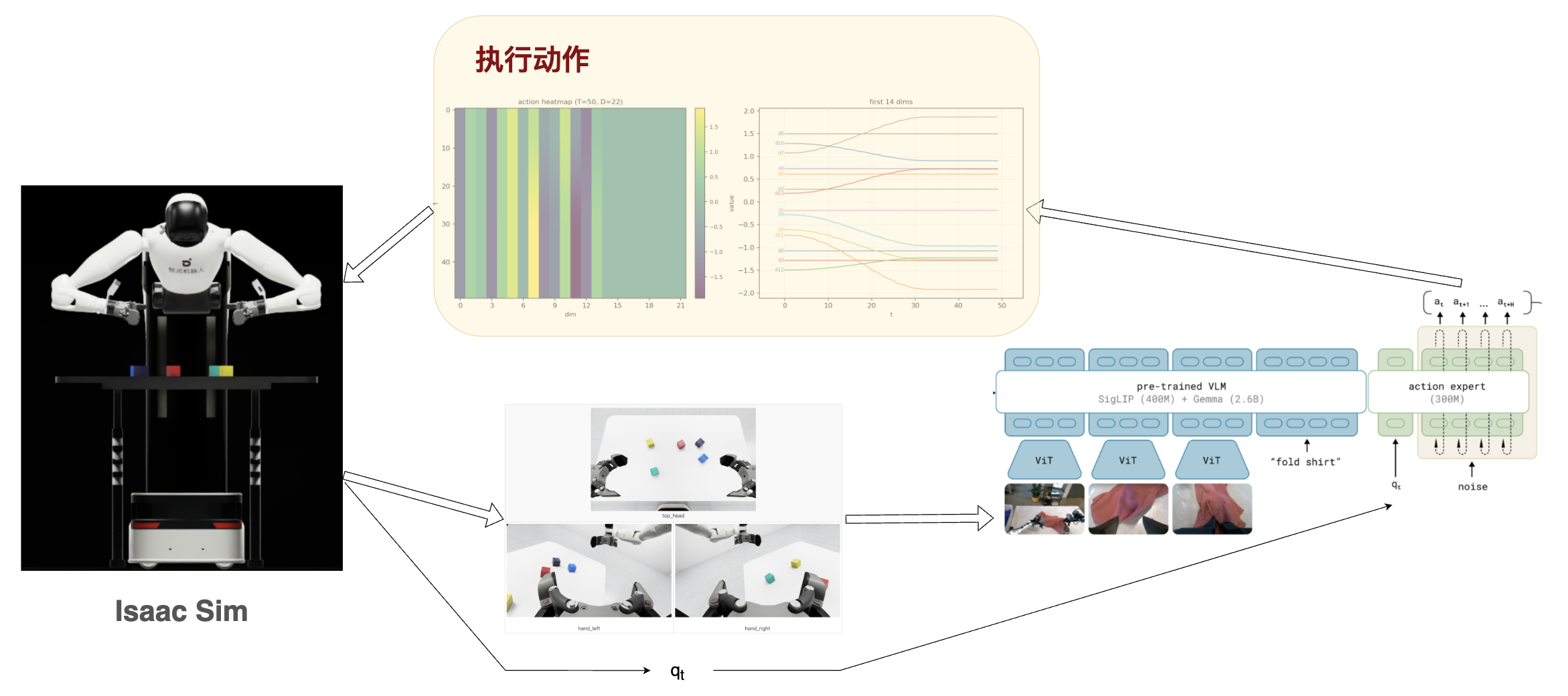
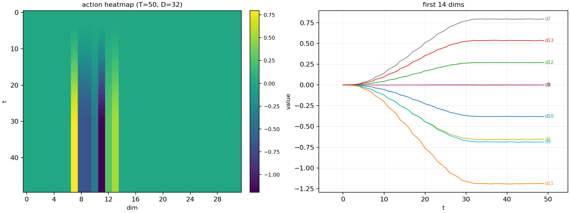
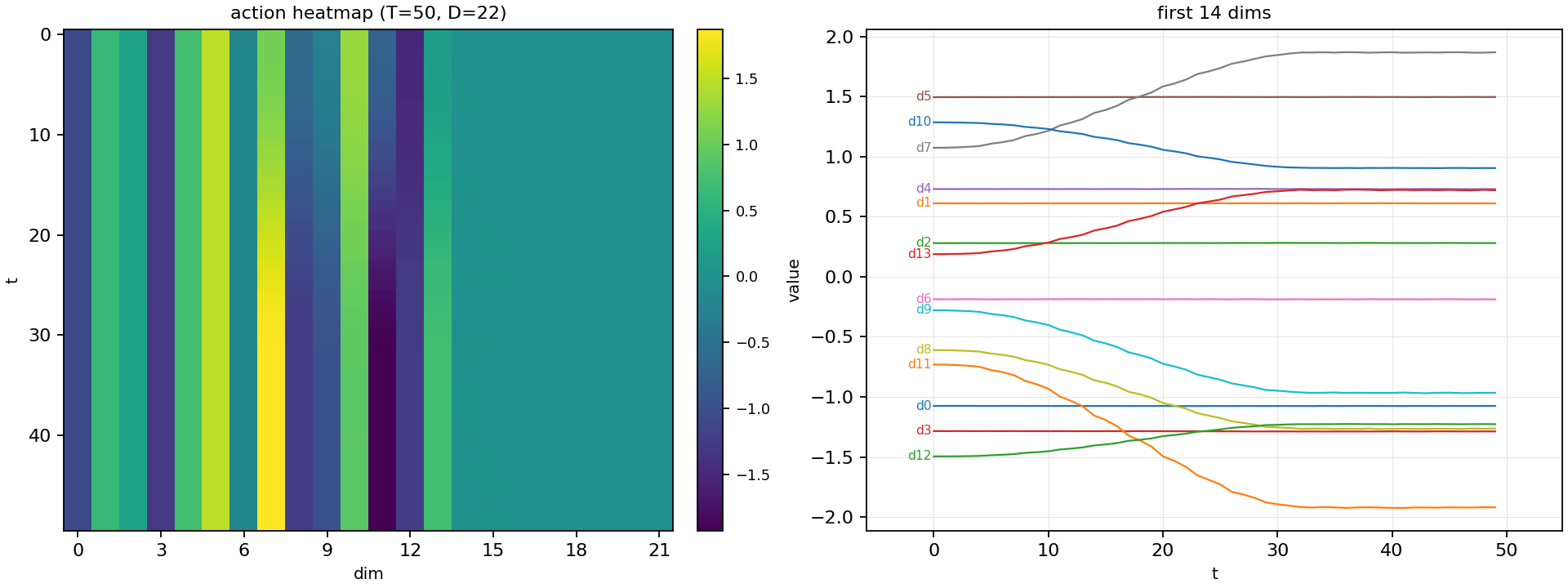
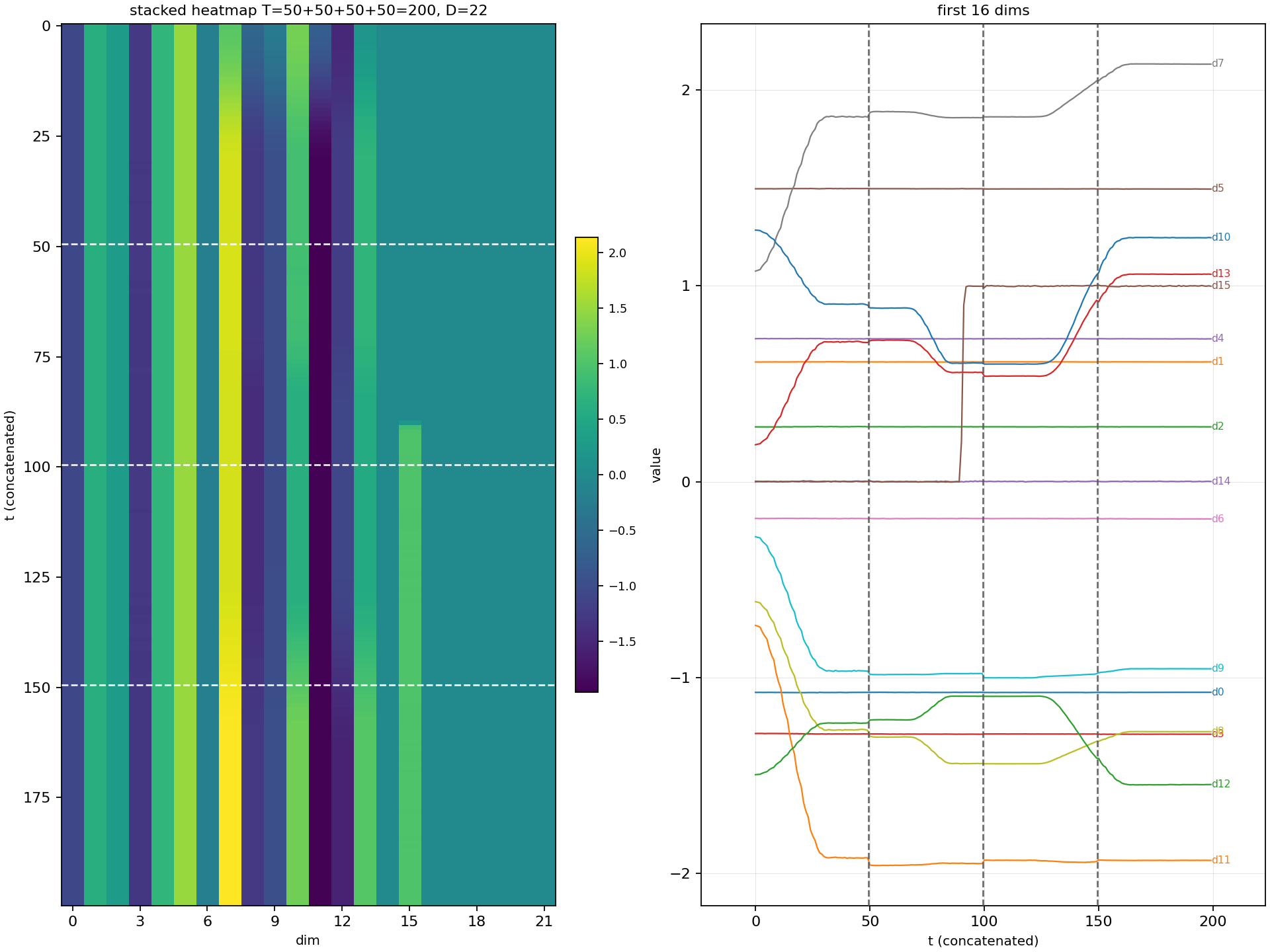
actions = torch.Size([1, 50, 32])
其中 50 是指 50 step,如果执行频率是 50 hz,则刚好是 1s 的动作规划。
32是
action_dim,本试验中用的只是前 22 维。
下图的变化,可以理解这是对各个关节接下来一秒的动作规划:
实际返回给仿真器的时候,是需要将这个 actions 与最初的 state 有选择的进行相加(夹爪不需要相加)。形成如下结果:
注意:模型生成的 action
是绝对的还是相对的,要看模型的配置。如果是绝对的则不用相加。
模型推理 (sample_actions) 拆解
进入本文的重点:sample_actions: Do a full inference forward and compute the action.
pi05 相关代码位于
src/lerobot/policies/pi05/modeling_pi05.py。这个模型对应
PaliGemmaWithExpertModel,整体可以概括为「VL
主干 + A 专家」两路协同:
paligemma(VL主干):负责视觉-语言理解与语义建模。视觉端先由SigLIP提取特征(1152 维),再通过projector映射到 2048 维,与语言分支(18 层、hidden size2048)对齐融合;gemma_expert(A专家):负责动作相关建模。层数与主干保持一致(18 层),但宽度降为 1024,并引入带条件输入的adaptive RMSNorm,使其成为更轻量、受主干条件引导的action expert。
如果想看完整模块展开,下面是直接打印出的 π0.5 结构:
展开查看完整 π0.5 模型结构打印
1 | self.paligemma_with_expert = PaliGemmaWithExpertModel( |
各个部分的计算量比例大概有多少呢?在Thor平台上进行部署 π0,各部分时间占用如下:
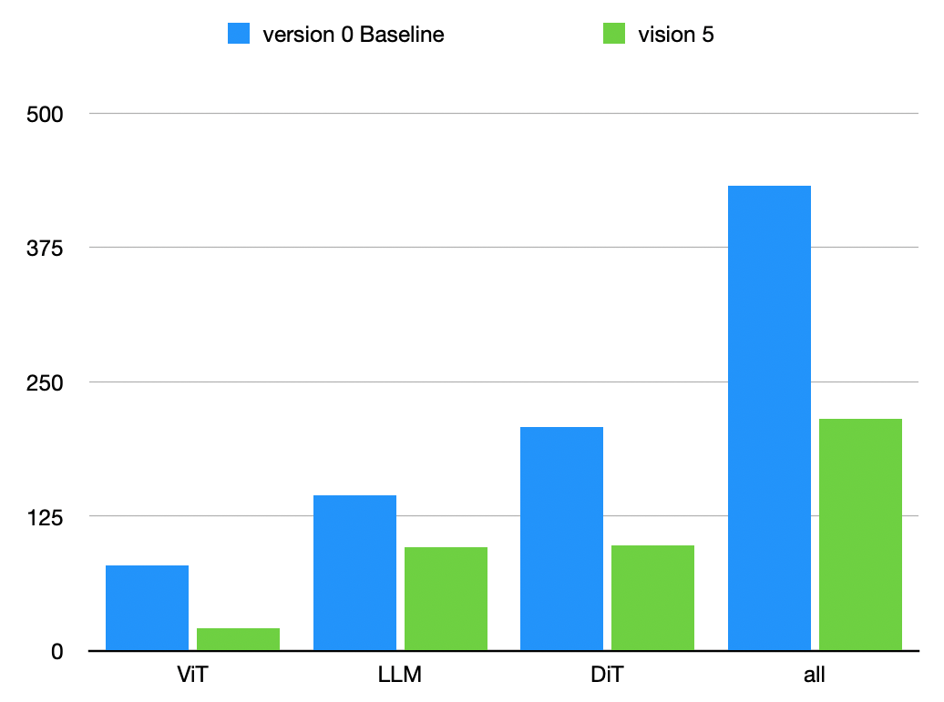
| Version | ViT (ms) | LLM (ms) | DiT (ms) | Total (ms) |
|---|---|---|---|---|
| Baseline | 79.38 | 144.70 | 208.12 | 432.20 |
| Optimized | 21.78 | 96.06 | 109.18 | 227.02 |
需要注意的是 DiT 的部分,模型虽然不大,但是它的 denoise 要循环 10 次,这导致了计算量的上升。
后续又做了进一步的优化,整体能在 190ms 左右。不过大体上还是这个比例。 π0.5 我还没有部署分析,不过应该也是这个比例和量级。
\(\mathrm{VLA}\) 之 \(\mathrm{V}\)iT 模块
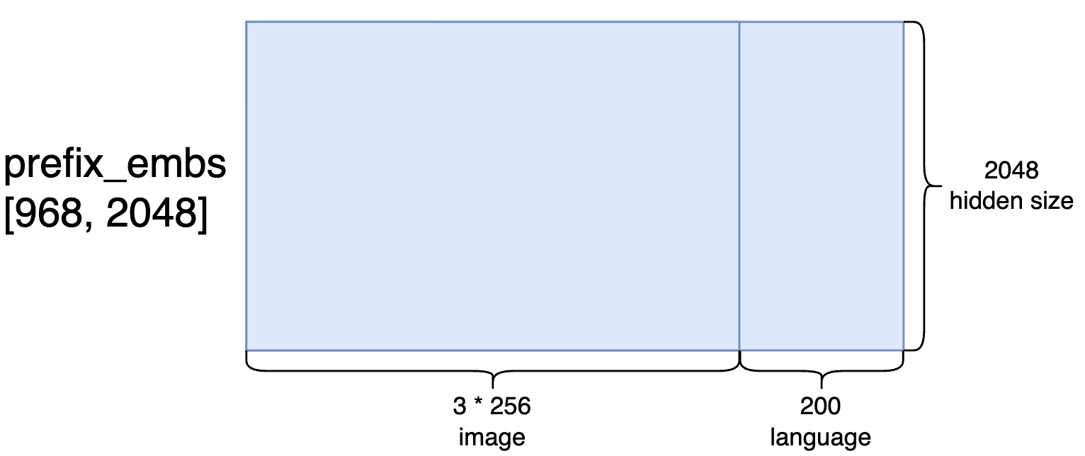
1 | prefix_embs, prefix_pad_masks, prefix_att_masks = self.embed_prefix(images, img_masks, tokens, masks) |
这个函数的作用是把 多路图像 + 文本 tokens 统一打包成 Transformer 前缀输入:
- 先分别做图像/文本 embedding,再在序列维拼接成
embs。 - 同时构造两类 mask:
pad_masks(哪些位置是有效 token)和att_masks(前缀可见性标记)。 - 最终返回
(embs, pad_masks, att_masks),供后续主干直接做前向推理。
伪代码:
1 | function embed_prefix(images, img_masks, tokens, token_masks): |
prefix_embs 的 shape 为 torch.Size([1, 968, 2048])
关于 SigLIP 的模型结构,第一层的卷积层可以稍微关注一下:
1 | (patch_embedding): Conv2d(3, 1152, kernel_size=(14, 14), stride=(14, 14), padding=valid) |
使用以前做的一个4图像输入的情况为例:
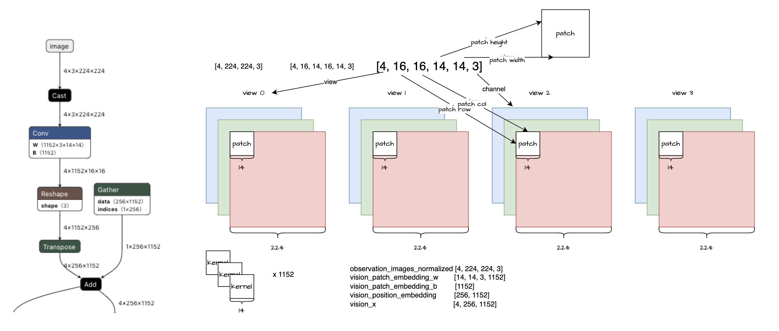
结论:这其实是个全连接,可以用全连接算子做加速。
SigLIP是 Google 提出的一个视觉-语言预训练模型(Vision-Language Model),全称可理解为Sigmoid Loss for Language-Image Pre-training。它和CLIP类似,目标都是把图像和文本映射到同一语义空间做对齐,但 SigLIP 用的是sigmoid/binary风格损失,而不是 CLIP 常见的softmax对比损失。在这里,SigLIP主要扮演 视觉编码器(ViT) 的角色:把输入图像变成语义特征,再交给后面的语言/动作模块继续处理。
这是一个比较成熟的提取图像特征的模型,本以为这里发挥的空间并不大,无非是分辨率从224改为448,后来看 \(\pi_{0.7}\) 的论文里提到
The history frames are processed through the vision encoder and compressed to the same number of tokens as a single frame
这个做法也是挺妙的。
还有一个明显的点可以进行推理优化:
在 embed_prefix 函数中对图像进行的是循环处理
1 | # Process images |
这里完全可以对图像进行组 batch
进行推理,经过实测这个优化可以极大地降低 ViT
部分的耗时。
关于 Vit 还有一个很大的陷阱: transformers 的 v5.4.0
以前,get_image_features 返回的是缩放后的的 feature。
1 | image_features = image_features / (self.config.text_config.hidden_size**0.5) |
v5.4.0 以后则取消了这个缩放。这其中的一个改变来自于其中的一个 commit
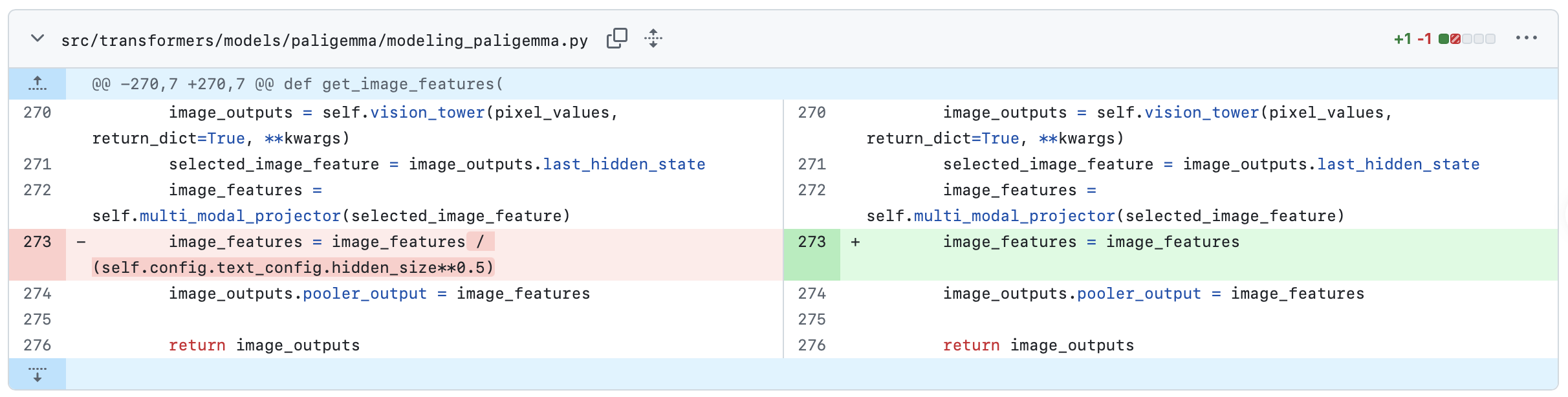
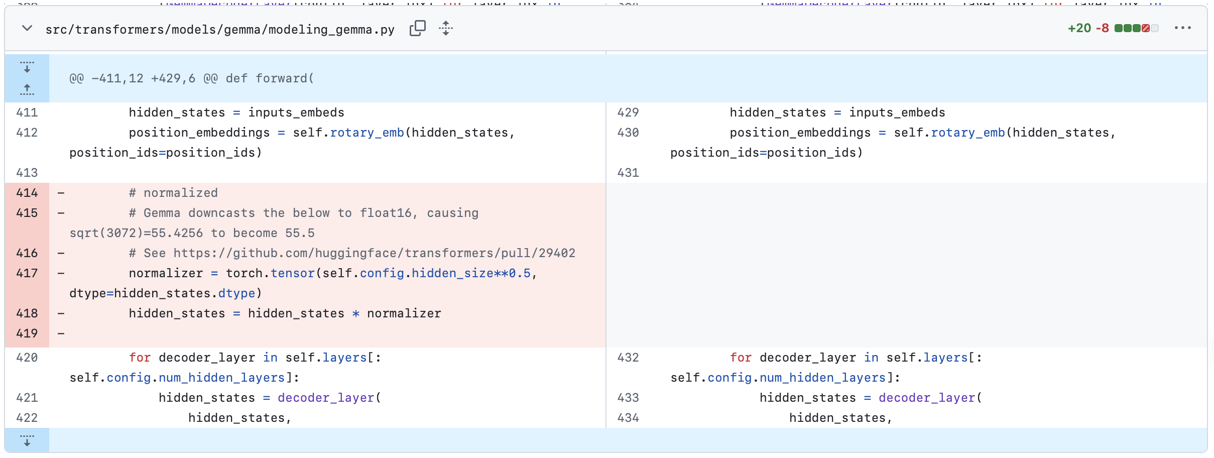
这会导致 transformers 的 v5.3.0 和 v5.4.0 的接口要求有数量级上的差异。如果transformers版本没有和缩放逻辑对齐,必定影响模型推理结果。
\(\mathrm{VLA}\) 之 \(\mathrm{L}\)anguage 模块
1 | _, past_key_values = self.paligemma_with_expert.forward( |
具体的 forward 是:
1 | if inputs_embeds[1] is None: |
这个就是一个正常的大模型推理,倒是没什么好进一步展开解释的。在本次试验中,输入长度是 968,所以输出为:
prefix_past_key_values- 共 18 layers, 每一层的 shape 都是一样的,均为
key: (1, 1, 968, 256)value: (1, 1, 968, 256)
- dtype=torch.bfloat16
- total KV storage ~17.02 MiB (all layers)
- 共 18 layers, 每一层的 shape 都是一样的,均为
prefix_output- torch.Size([1, 968, 2048])
- dtype: torch.bfloat16
需要注意的是,如果不使用 π0.5 及以后版本的 subtask
的话,prefix_output 和 prefix_past_key_values
的第 18 层是不需要计算的。这样可以节省不少计算量。
输出的 prefix_past_key_values 与
action expert 模块通过 kv kache 交互,即
Cross-Attention。
输出的 prefix_output 可用于做 RL Token。
\(\mathrm{VLA}\) 之 \(\mathrm{A}\)ction 模块
降噪过程动图如下:
动图为左 / 中 / 右三列对齐的可视化,含义如下。
- 左列 \(x_t\):当前步 Euler 更新之前的状态,即整块 action 的噪声 / 中间量在 (50×32) 网格上的强度。
- 右列 \(|v_t|\):策略给出的速度场模长。
- 中列:与左右相同分辨率;在每个局部块内把速度 \(v\) 投影成二维向量,再乘以步长 \(dt\) 得到位移箭头场。离散意义上 \(\Delta x \approx dt \cdot v_\theta(x,t)\),用来直观表示 flow matching 里「沿学到的向量场,把样本从噪声端往数据端推」的那一步。
时间方向:由 \(t\approx 1\) 走向 \(t\to 0\)。最后一帧会补上由 \(x + dt\cdot v\) 得到的终态,与模型里真实的 Euler 更新一致。
Action 是流匹配 /
扩散式的生成:实现里对带噪动作做固定次数的离散更新,本配置典型为
10 步(与主循环里 denoise
迭代次数一致),每一步都在「当前噪声动作 +
当前时间标量」条件下调用 Gemma 动作专家(action
expert)。
在每一步送进专家主干之前,需要先把
(noisy_actions, timestep) 整理成专家可做自注意力(并与 VLM
prefix 做 Cross-Attention)的输入,主要包括:
- Token 嵌入:噪声动作经线性投影后的 suffix 序列表示;
- Padding 掩码:哪些位置是有效 token;
- 注意力掩码:suffix 与 prefix 之间的可见性(配合已缓存的 VLM KV);
- AdaRMS 条件:由时间步嵌入经小 MLP 得到,用于在专家层内做自适应归一化调制。
下面从 embed_suffix 按代码拆解(suffix
即相对图像+语言前缀之后的第二段序列)。
1 | def embed_suffix(self, noisy_actions, timestep): |
时间步嵌入
时间标量
timestep先被编成固定维向量,再经浅层 MLP 得到adarms_cond:前半段类似 Transformer 里的正弦–余弦位置编码(多频、平滑),后半段把该几何特征压成更适合作为 AdaRMS 条件的向量,使专家在去噪轨迹的不同位置有不同的归一化尺度与偏移。1
2
3
4
5
6
7
8# Embed timestep using sine-cosine positional encoding
time_emb = create_sinusoidal_pos_embedding(
timestep,
self.action_in_proj.out_features,
min_period=self.config.min_period,
max_period=self.config.max_period,
device=timestep.device,
)create_sinusoidal_pos_embedding:把timestep映射到与action_in_proj.out_features相同维度的向量,语义上表示「当前处于去噪过程的哪一段」;min_period/max_period控制频谱覆盖,避免只在单一尺度上对 (t) 敏感。- 形状示例:
time_emb.shape == torch.Size([1, 1024])(首维为 batch,与下文action_emb的隐藏维一致,便于与动作分支对齐)。
1
2
3
4
5
def time_mlp_func(time_emb):
x = self.time_mlp_in(time_emb)
x = F.silu(x)
x = self.time_mlp_out(x)
return F.silu(x)time_mlp_func:Linear → SiLU → Linear → SiLU,即两层 MLP;输出即送入专家各层的adarms_cond(与「把时间信息直接加到 token 上」不同,这里主要通过 AdaRMS 调制层内统计量,把 (t) 信息注入主干)。
动作嵌入
noisy_actions一般为[B, T, D_a]:(T) 为动作 horizon(如 50),(D_a) 为单步动作维(如 32,即max_action_dim)。先经action_in_proj(由_apply_checkpoint包一层以省显存)线性映射到专家隐藏维,得到 suffix 上的action_emb。时间信息不在这一步与 token 特征相加,而是单独走adarms_cond,经 AdaRMS 注入各层。1
action_emb = self._apply_checkpoint(action_proj_func, noisy_actions)
- action_in_proj(noisy_actions):把噪声动作(最后一维一般是
max_action_dim)线性投到专家隐藏维,得到 action_emb。
- 作为 suffix 序列的 token 表示
- 这里还没和 time 在特征维上相加
- noisy_actions.shape: torch.Size([1, 50, 32])
- action_emb.shape: torch.Size([1, 50, 1024])
1
2
3
4
5
6
7
8outputs_embeds, _ = self.paligemma_with_expert.forward(
attention_mask=full_att_2d_masks_4d,
position_ids=position_ids,
past_key_values=past_key_values,
inputs_embeds=[None, suffix_embs],
use_cache=False,
adarms_cond=[None, adarms_cond],
)outputs_embeds.shape: torch.Size([1, 50, 1024])
1
2
3
4suffix_out = outputs_embeds[1]
suffix_out = suffix_out[:, -self.config.chunk_size :]
suffix_out = suffix_out.to(dtype=self.action_out_proj.weight.dtype)
return self.action_out_proj(suffix_out)[:, -chunk_size:]:当 horizon 大于chunk_size时,只保留最后chunk_size个时间步上的隐状态,与「动作块」预测窗口对齐(chunk_size与配置里Pi0Config等一致)。action_out_proj:线性头把隐藏维投回action_dim,得到本步网络对速度场 / 噪声等目标的预测;形状示例:torch.Size([1, 50, 32])(与noisy_actions末维一致)。
- action_in_proj(noisy_actions):把噪声动作(最后一维一般是
max_action_dim)线性投到专家隐藏维,得到 action_emb。
具体的 forward 是:
1 | elif inputs_embeds[0] is None: |
进行多次推理,得到一个完整的动作序列:
对应的仿真里面机器人的运动轨迹:
其他
模型配置
模型使用了 select_color,不过这是 OpenPI 的 JAX 格式,我倾向于用 LeRobot 进行推理,于是进行格式转换:
1 | (openpi) python3 examples/convert_jax_model_to_pytorch.py \ |
我当前 LeRobot 的版本是 1
2
3commit 720cf8e3a09f62fa95260cc49a7a30e5d0f7473a (HEAD -> main, origin/main, origin/HEAD)
Author: Steven Palma <imstevenpmwork@ieee.org>
Date: Mon Mar 30 19:11:41 2026 +0200
注:OpenPI的代码逻辑和LeRobot的代码逻辑和实现有差异,直接替换的话完全不work,需要做一些修正(RoPE)。
1 | (lerobot) x@portal:~/Desktop/lerobot$ lerobot-info |
看各家模型结构的设计很有意思,能看出使用各种技巧
比如 GR00T 的模型结构(这图画的要比pi0清晰一些)
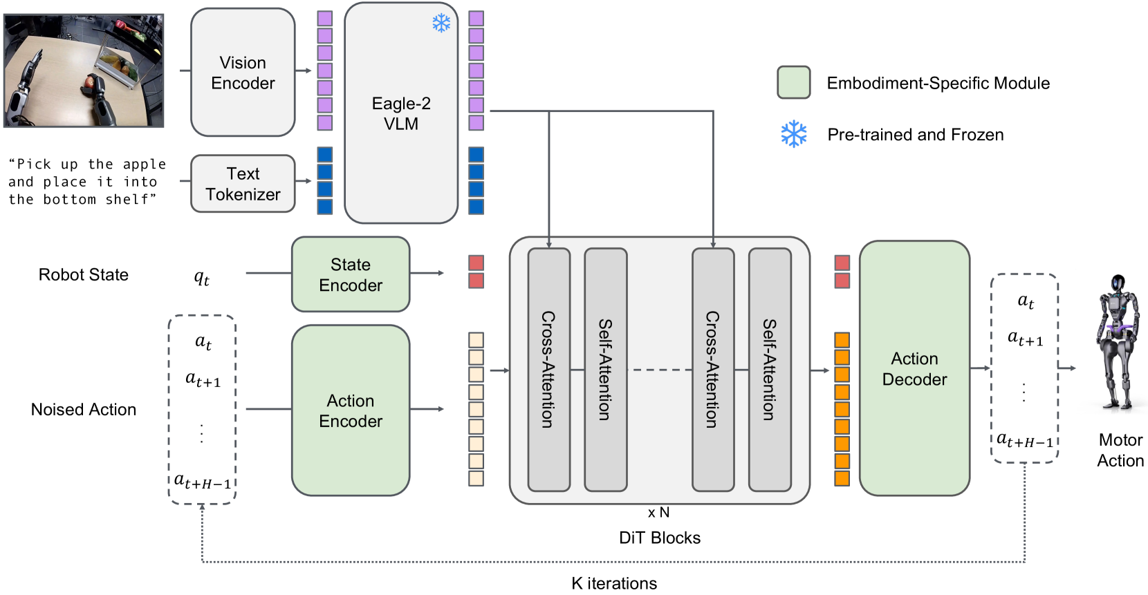
pi07的模型结构
画图运行脚本:
1 | (lerobot) x@portal:~/Desktop/serve_lerobot$ python serve_lerobot_pi05.py |
src/lerobot/policies/pi05/README.md
| Feature | π₀ | π₀.₅ |
|---|---|---|
| Time Conditioning | Concatenates time with actions via
action_time_mlp_* |
Uses time_mlp_* for AdaRMS conditioning |
| AdaRMS | Not used | Used in action expert |
| Tokenizer Length | 48 tokens | 200 tokens |
| Discrete State Input | False (Uses state_proj layer) |
True |
| Parameter Count | Higher (includes state embedding) | Lower (no state embedding) |
以上就是前段时间对 π 的探索和实践,整理得有些乱七八糟,不过该记录的都记录了,以后有时间再进一步完善。欢迎讨论 :-)